
All content Copyright 2022 Parallel Systems Ltd.
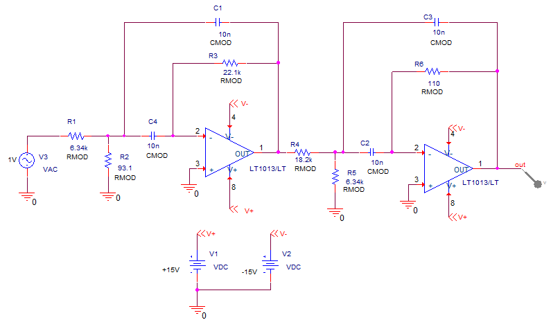
A typical application of Monte Carlo analysis is predicting yields on production runs of a circuit board. Probe can be used to display data derived from Monte Carlo waveform families as histograms, which is part of Probe’s performance analysis feature.
This Chebyshev filter is designed to have a 10kHz centre frequency and a 1.5 kHz bandwidth. The components were rounded to the nearest available 1% resistor and 5% capacitor values. In our analysis, we are concerned with how the bandwidth and the centre frequency vary when 1% resistors and 5% capacitors are used in the circuit.
As in the last exercise, we would need to create models for the devices we wish to vary, in this case, the resistors and capacitors. The models are defined as:
.model RMOD RES R=1 DEV=1%
.model CMOD CAP C=1 DEV=5%
Alternatively, since these models are using only the DEV tolerance, you can use the standard R and C parts and simply supply values for the Tolerance property.
(This has already been configured in the project that will be used for this lab)
To analyze the filter, an AC analysis with a Monte Carlo analysis will be configured. The AC analysis sweeps 50 points per decade from 100Hz to 1 MHz and the Monte Carlo analysis is set to take 100 runs. The output variable of interest is V(OUT).
The data file can become quite large when running a Monte Carlo analysis. Since only the output of the filter is of interest, a voltage marker will be placed at the output, and then the simulation set up to collect data at the marked node only.
1. Open the provided Cheby project from the C:\OrCAD_Training\PSpice directory.
2. Run the simulation.
The Probe window opens, select all the results and the output response will be displayed (because of the Voltage probe at the OUT node)
3. Left-click on the V(out) trace name in the Probe Window and use delete to remove the traces.
4. Left-click the Performance Analysis toolbar button.
5. Left-click the Add Trace toolbar button, or use Trace>Add Trace from the top menu.
The following 4 steps describe one way of quickly generating the desired trace expression. You may also just type in the entire expression as documented in step 8.
6. Select the Bandwidth(1,db_level) function from the Functions or Macros section.
7. Without moving the insert cursor, left-click on the V(out) trace name.
8. Without moving the insert cursor, type 1.
9. Move the cursor to after the V and insert db.
The trace name is now Bandwidth(Vdb(OUT),1)
(The bandwidth between the two 1dB levels of V(out))
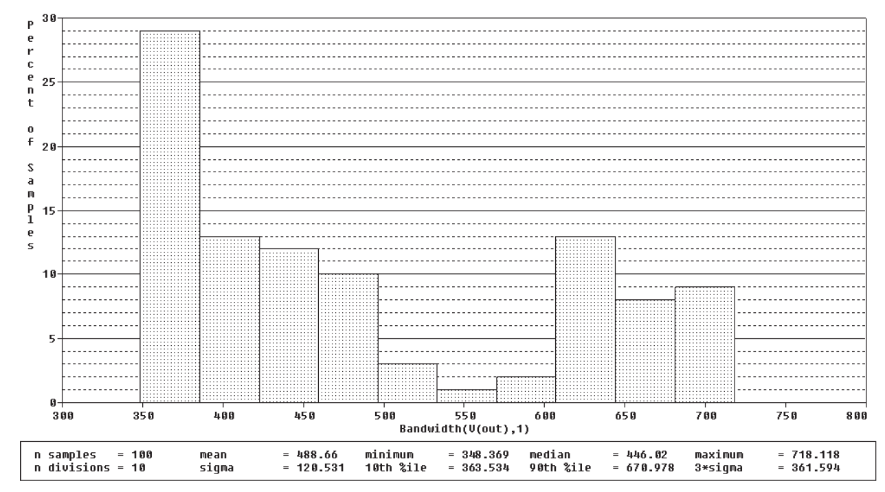
10. Left-click>OK to view the histogram.
Since a Monte Carlo analysis is random, your results may vary slightly from those shown in the following graphic
11. Select Tools>Options from the top menu and enter 20 in the Number of Histogram Divisions text box.
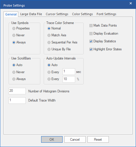
12. Left-click>OK.
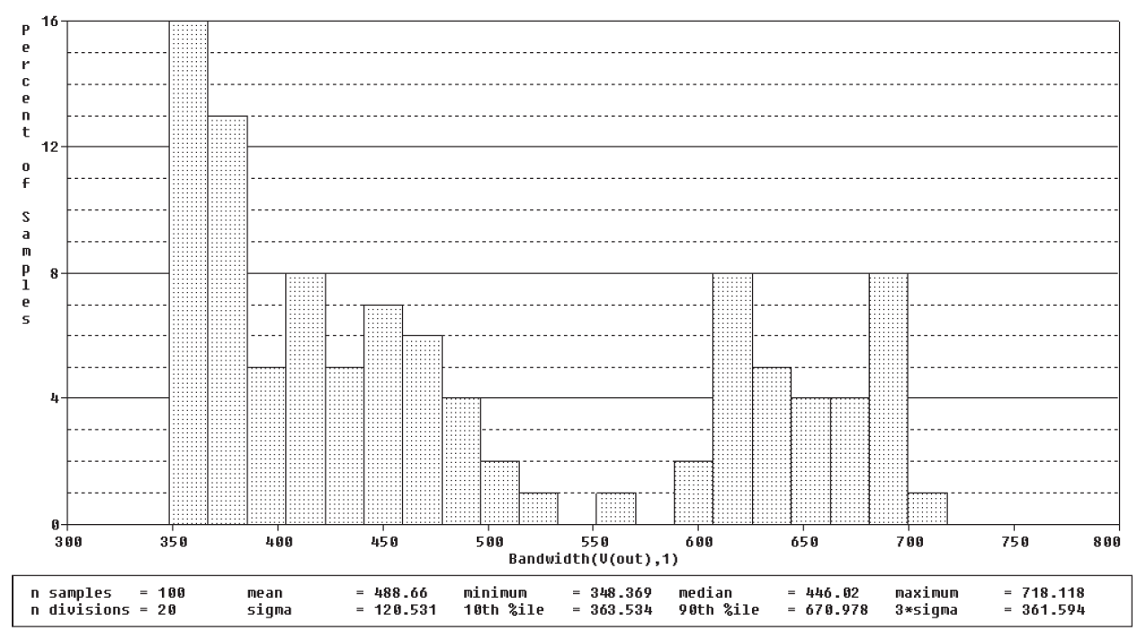
The statistics for the histogram are displayed by default. However, this may be turned off by choosing Tools>Options and then deselecting Display Statistics.
13. Left-click the Add>Trace toolbar button, or select Trace>Add Trace from the top menu.
14. Select the CenterFreq(1, db_level) function by left-clicking on it.
15. Select V(out) by left-clicking on it.
16. Edit the Trace Command box to read CenterFreq(Vdb(OUT),1).
17. Left-click>OK to view the histogram.
The new histogram replaces the old one.
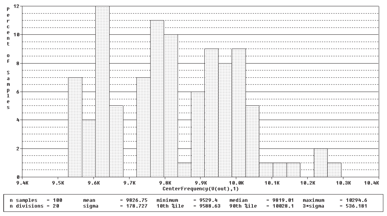
To view both simultaneously, choose Plot>Add Plot to Window before adding a new trace. The histogram for centre frequency is shown in the graphic that follows.
Additional Exercise
Experiment with creating histograms using the Centre Frequency and Bandwidth functions when the dB level is changed from 1 to 3.
Experiment with other Performance Analysis functions.

End of Lab
All content Copyright 2022 Parallel Systems Ltd.
Additional Exercise (Optional)
Another Bandpass filter implementation is provided for investigation. This uses fewer components so it could be possible that “less is more”
1. Open the bandpass2 project from the C:\OrCAD_Training\PSpice directory.
This is configured with the same component tolerances and simulation profile as the previous lab, 1% resistors and 5% capacitors.
2. Run the simulation and examine the results.
3. Delete the default Vdb(out) trace from the probe in the schematic and use the Performance Analysis toolbar button to examine the Bandwidth and Centre Frequency.
(Refer to the previous section of this lab for a reminder of the process)
Use levels of 1dB and 3dB to get some comparison of the performance and yield to the 10kHz centre frequency and 1.5kHz bandwidth specification.
(A web site calculator was used to get the circuit topology and component parameters for this section)
All content Copyright 2022 Parallel Systems Ltd.