
All content Copyright 2022 Parallel Systems Ltd.
To complete the steps in this lab, continue using the RC project you created in lessons 1 and 2.
1. Select PSpice>New Simulation Profile from the top menu, or left-click the New Simulation Profile toolbar button.
2. Name the new simulation profile RC_DC and left-click on Create.
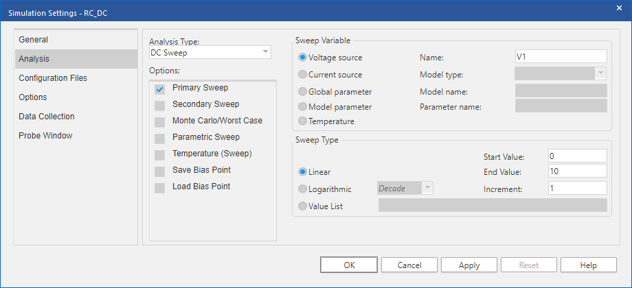
3. Left-click Analysis on the left hand side.
4. From the Analysis Type drop-down choose DC Sweep.
5. In the Options section only Primary Sweep should be highlighted and checked.
6. In the Sweep Variable section check Voltage Source.
7. Type V1 in the Name field.
8. In the Sweep type section check Linear.
9. Enter 0 in the Start Value field.
10. Enter 10 in the End Value field.
11. Enter 1 in the Increment field.
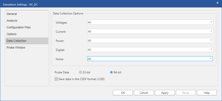
12. Left-click Data Collection on the left hand side.
Data collection settings for voltages, currents, power, digital, and noise display.
13. From the drop-list menus of each option, select All.
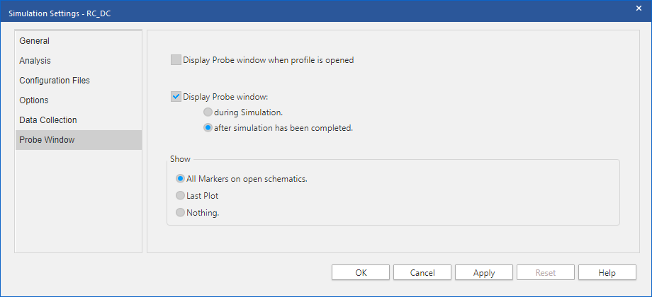
14. Left-click Probe Window on the left hand side.
15. Check the option, Display the Probe Window after simulation has completed.
16. Check the option, Show: All markers on open schematics.
17. Left-click>OK to close the Simulation Settings dialog box.
18. From the schematic view, choose PSpice>Run or left-click on the Run toolbar icon to run the simulation.
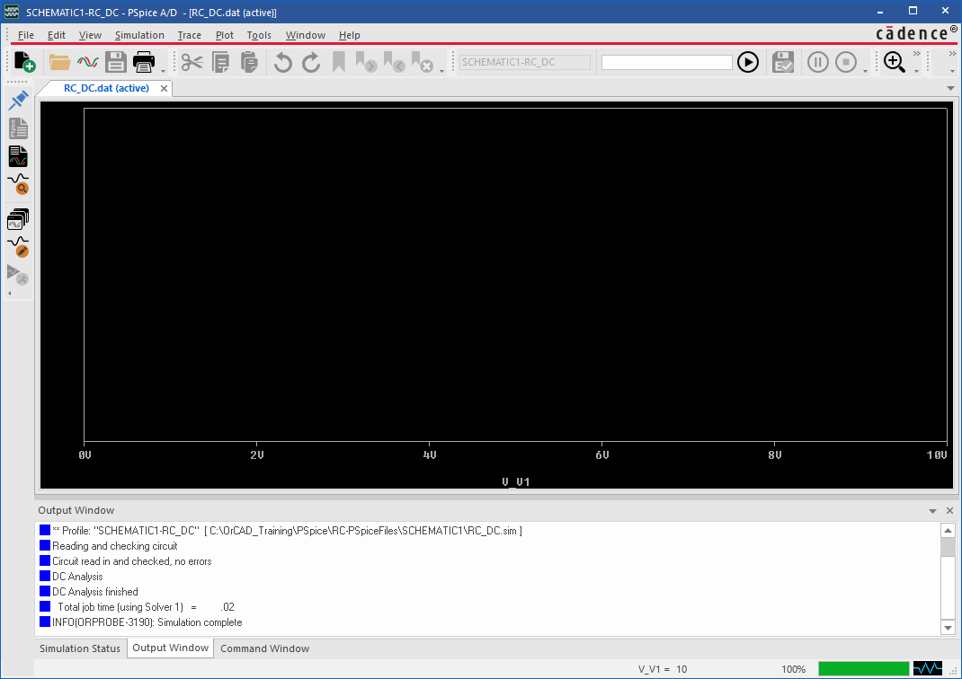
The system automatically generates the netlist and runs the simulation. When the simulation run is complete the Probe windows opens.
When the Probe window appears, you are presented with a blank plot screen. If you have used markers in the design, then you will see the traces for those markers already displayed.
19. From the Probe window, choose Trace>Add Trace or left-click on the Add Trace icon. The Add Traces dialog opens.
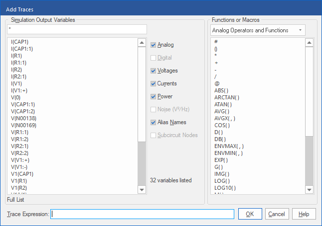
20. Left-click on the V(IN) and V(OUT) entries in the Add Trace list to select them, this will add the selected trace names to the Trace Expression field at the bottom of the window. All traces listed in the Trace Expression field will be displayed at the same time.
21. Left-click>OK to display the selected traces, similar to the next graphic:
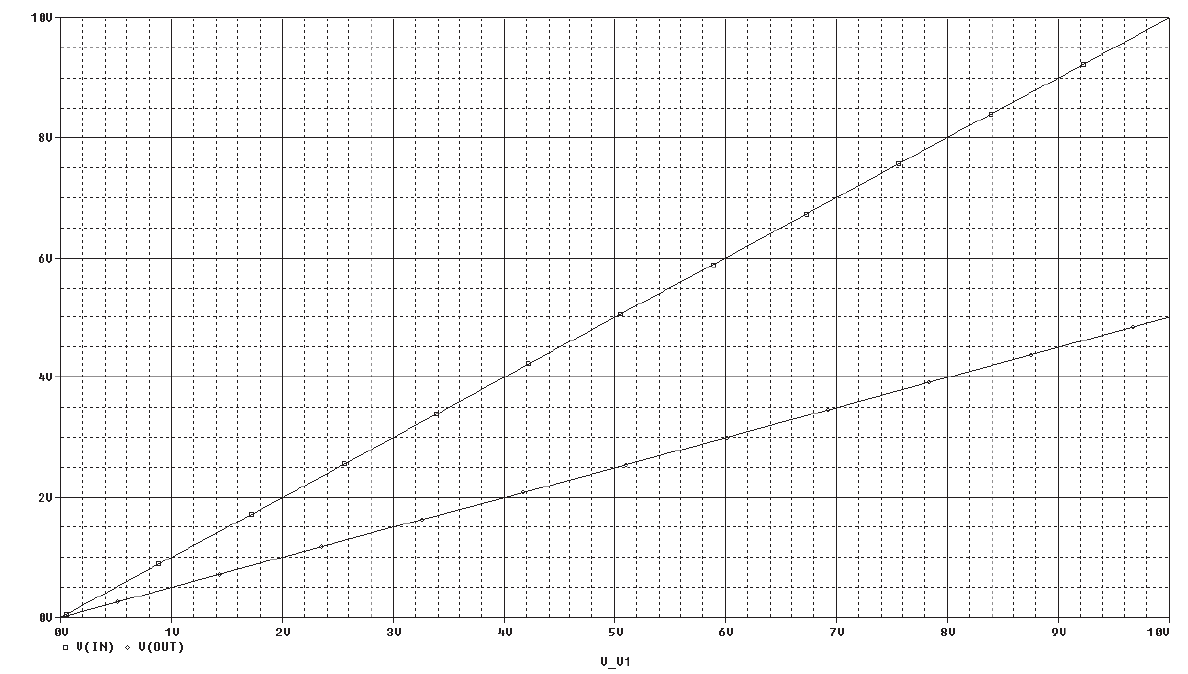
To see how markers display traces in the Probe window, delete the two displayed traces and add them back in using markers as described in the steps that follow.
22. Left-click on the trace name V(IN) located below the X axis.
The colour of the trace name changes (to red) indicating it is now selected.
23. Press the Shift key and left-click on the V(OUT) trace name.
The colour of this trace name also changes (to red) indicating that it also selected.
24. Press the Delete key to remove both traces from the display.
25. Press Alt+Tab to switch back to the Capture window, or left-click on the Capture task bar icon.
Check that the Schematic Page is open, if necessary, select the tab for the Schematic page to activate it.
26. Choose the PSpice>Markers>Voltage Level menu commands.
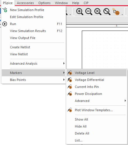
The Voltage Level marker attaches to the mouse cursor.
27. Move the mouse to the IN wire and left-click on the wire to place the marker.
28. Move the mouse to the OUT and left-click on that wire to place a second marker.
29. Press Esc, or right-click>End Mode, to exit the Voltage marker placement command.
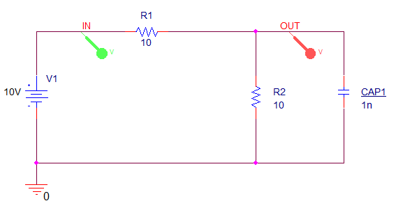
With the Probe window open, the Voltage markers will be assigned the trace colours.
30. Return to the Probe window to view the graphic display of the traces you just added.
(Alt+Tab, or select the Task Bar icon)
The appearance of the Probe window can be changed to a great extent. Trace colours can be changed, grid spacing can be modified, trace symbols can be changed or displayed.
31. From the Probe window, left-click a trace, or its symbol located below the X axis using your right mouse button.
32. From the pop up menu that displays, choose the Trace Property menu option.
The Trace Properties dialog box opens.
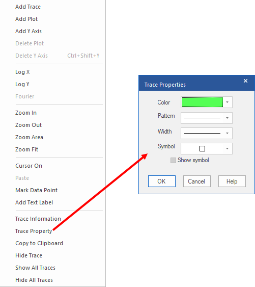
33. Change the colour setting of the trace, the pattern of the line, the thickness of the line, the symbol denoting the trace, and whether or not to display the symbol on the trace itself.
34. Left-click>OK to save your changes and close Trace Properties
Note:
The Symbol display on the traces is controlled from Tools>Options, General tab, Use Symbols group, “Always” is set as the default, this needs to be changed to “Properties” so that the Trace Symbol display will be controlled from the Trace Properties settings.
35. To edit axis and grid settings, right-click on any of the grid lines and choose Settings from the menu presented. Or, select Plot>Axis Settings from the Probe window top menu.
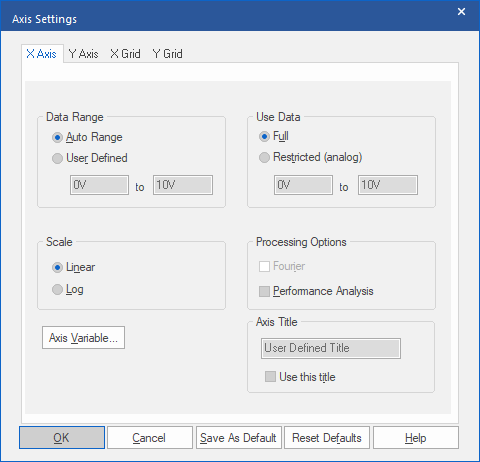
36. Left-click the X Axis to open a tab that enables you to:
Set the displayed data range.
Set the range of data that Probe functions consider.
This is useful when making a Fourier plot since you will want an integral number of cycles or perhaps data from only the last portion of the simulation after the circuit has settled.
Specify whether the scale should be Linear or Logarithmic.
Enable the Fourier mode or Performance Analysis mode.
Change the X axis variable.
37. Left-click the Y Axis to open a tab that enables you to:
Set the Data Range that will be displayed.
Specify if the scale should be Linear or Logarithmic.
Change the axis title.
Change the axis number.
38. Left-click on the X Grid to open a tab that enables you to:
Set the major grid spacing.
Choose the way in which the grids will be drawn (lines / dots / + symbols.)
Choose to display numbers below the axis.
Choose to display tick marks inside the plot edge.
Chose the minor grid spacing.
Chose the way the grid will be drawn
Choose to display tick marks inside the plot edge.
39. Left-click the Y Grid to open a tab that enables you to:
Set the major grid spacing.
Choose the way in which the grids will be drawn (lines / dots / + symbols.)
Choose to display numbers below the axis.
Choose to display tick marks inside the plot edge.
Chose the minor grid spacing.
Chose the way the grid will be drawn
Choose to display tick marks inside the plot edge.

End of Lab
All content Copyright 2022 Parallel Systems Ltd.