All content Copyright 2022 Parallel Systems Ltd.

 

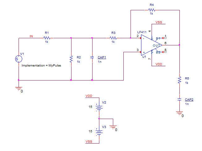
1. Open the Buffer project and the open the schematic page.

 

2. Left-click the Place Part button, or select Place>Part from the top menu

 

3. Type Param in the Part field of Place Part.

 

4. Left-click to select the part and press Enter, or double-click the part to attach the part to the cursor.

 

5. Left-click in the schematic page to place the Param symbol.

 

6. Press Esc, or right-click>End Mode, to end the placement command.

 

7. Double-click on the Param part just placed to open the Property Editor tab.

 

8. Left-click the New Property button.

 

9. Name the property CVAL, set the Value to 1n, left-click the Display On / Off box and left-click>OK to set the Property and Value.

 

10. In Display Properties form that is displayed, set the Display option to Name and Value and left-click>OK to accept.

 

11. Left-click in the Property Editor tab, at the top, and right-click>Close

This defines the global parameter CVAL, assigns it a default value of 1n, and sets the display to show both the property name and value. At this point it is still not being used by any device and would have no affect on simulation.

 

12. Double-click the value of CAP2, currently 1n to open the Property Editor

 

13. Type {CVAL} as the new value. The curly braces are required here.

 

14. Left-click>OK to set the value.

Any time a model parameter or component value (as in discrete components like resistors, caps, and inductors) is to be assigned at the time of simulation, it is enclosed in curly braces { }. This tells PSpice to evaluate the variable or expression rather than using some preset value. For instance, if CAP2 from the last example is given a “value” of {CVAL} instead of 1n, PSpice will look for a global variable called CVAL and will substitute the current value of CVAL for the default value of the capacitor.

 

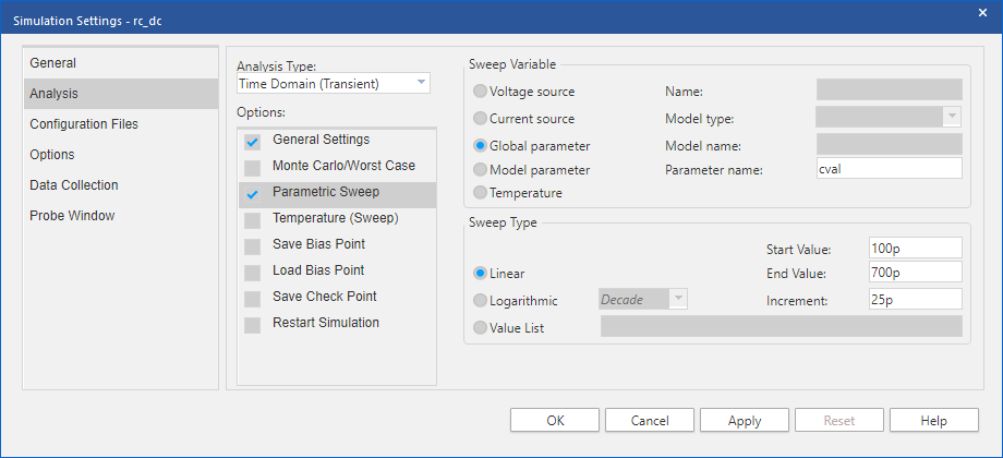
15. Edit the simulation profile.

 

16. Left-click Analysis on the left hand side and left-click the Parametric Sweep option.

 

17. Check the Global Parameter radio button. This will highlight all of the necessary fields.

 

18. Type CVAL in the Parameter Name field.

Note that it is not enclosed in curly braces.

 

19. Select the Linear radio button in the Sweep type section of the dialog.

 

20. Set the Start Value to 100p for this exercise.

 

21. Set the End Value to 700p for this exercise.

 

22 Set the Increment to 25p.

 

23. Confirm that Time Domain (Transient) is the selected analysis type.

 

24. Left-click>OK to save the changes and close the simulation settings.

 

25. Run the analysis.

 

26. Since there are 25 runs of the transient analysis, each with a different value of CAP2, the simulation will complete and display an Available Sections window listing all 25 runs with the value of CVAL for each run. There is the option to select which runs to view, use, left-click>OK to take the default of “all” sections.

 

27. Select Trace>Add Trace from the top menu, or use the Add Trace toolbar button.

 

28. Select I(CAP2) from the list of traces.

 

29. Left-click>OK to close the Add Trace window.

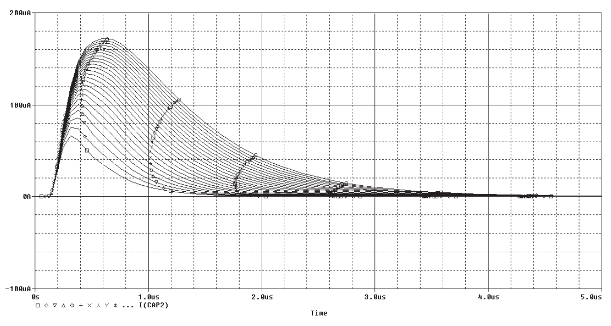
All 25 traces will be displayed.

If there had been a current marker on the input pin of CAP2, then the same family of curves would have been displayed from the schematic.

Now let’s compare the current through CAP2 for the first run where CAP2 is set to 100p and the last run where is it set to 700p.

 

30. Left-click I(CAP2) below the X axis and press Delete to remove all 25 traces.

 

31. Select the Add Trace toolbar button, or Trace>Add Trace

 

32. Type I(CAP2)@25 I(CAP2)@1 in the trace command box separated by a space.

Set the I(CAP2) value by left-clicking on the I(CAP2) entry from the trace list and then typing the @<run> after it, then add another I(CAP2) and type the @<run> after the trace name. Left-click>OK to add the traces.

Notice the difference at the peak value. To quantify the change, the difference of the waveforms for runs 25 and 1 can be plotted and the search commands available in Probe can be used to find the exact peak.

 

33. Left-click the Add Trace toolbar button.

 

34. Type the waveform expression I(CAP2)@25 – I(CAP2)@1 in the trace command field. (Or build this by left-clicking the I(CAP2) trace entry and edit the expression)

 

35. Left-click>OK.

 

36. Left-click the Toggle Cursor toolbar button.

 

37. Left-click on the trace symbol in the legend representing the waveform expression I(CAP2)@25 – I(CAP2)@1.

 

38. Left-click on the Cursor Peak toolbar button.

(Peak is found by solving a mathematical expression for a rate of change of 0, so it is possible that the cursor will find a couple of “false” peaks before the “obvious” peak in the waveform, left-click the cursor peak icon to move to the next peak)

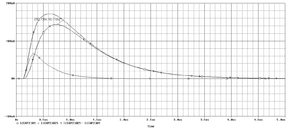
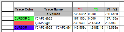
The above figures show the traces after the cursor has been placed at the peak and the values reported in the cursor window. Notice that the Y value in the cursor box is 143.559u. This tells you that when CAP2 is set to 700pF, the current through CAP2 is 144uA larger than when CAP2 is set to 100pF.

Probe provides a powerful technique for comparing characteristics of a family of waveforms called Performance Analysis (or Measurements). This uses search commands to define functions that detect points on each curve in the family. Once these functions have been defined in an external file, they can be applied to a family of waveforms through the standard Add Trace command, and produce traces that are a function of the variable that changed within the family.

 

In this example, it would be possible to apply a function using our search command to detect peak current for each waveform, then plot the peak versus the stepped CAP2 capacitance.

 

Refer to the PSpice A/D User’s Guide, the Probe online help, or the performance analysis wizard in Probe for additional help.

 

 

End of Lab

 

 

 

All content Copyright 2022 Parallel Systems Ltd.