All content Copyright 2022 Parallel Systems Ltd.

 

1. Open the provided Pressure project from the C:\OrCAD_Training\PSpice directory.

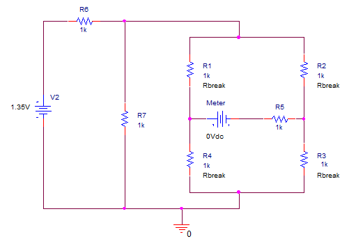
For reference the circuit uses the following items: Vdc, R (for R5-R7), 0, Param, Rbreak (R1-R4)

 

2. Check the properties of the Vdc part located in the bridge for a Value of 0 and a Reference of Meter.

Note

A zero volt, voltage source can be used as a current meter and a zero amp, current source can be used as a voltmeter in PSpice.

 

3. Left-click R1 to select it then right-click and choose Edit>PSpice Model to open the Model Editor.

 

4. Edit the model definition to be:

.Model Rmonte1 RES R=1 DEV=2% LOT=10%

 

5. Select File>Save from the Model Editor top menu to save the library file, the name should default to Pressure.lib to match the name of the source project.

 

6. Select File>Exit from the Model Editor top menu to close the Model Editor.

The <Implementation> property for R1 will change from the default Rbreak to the new RMonte1

 

7. Double-click on the <Implementation> (Rbreak) property for R2 and set the value to RMonte1.

 

8. Repeat step 7 for R3, and R4.

 

9. Place a Param symbol in the schematic and double-click it to edit the properties.

 

10. Left-click the New Property button.

 

11. Add the new properties named Pnom, P, and Pcoeff with values as follows:

Pnom = 1.0

P = 0

Pcoeff = -0.06

 

12. To display Param properties and values on the schematic page:

a) Highlight a the value cell (either Pnom, P, or Pcoeff) in the Property Editor.

b) Left-click the Display button in the Property Editor

c) Select the Name and Value display option in the Display Properties dialog box and left-click>OK.

 

 

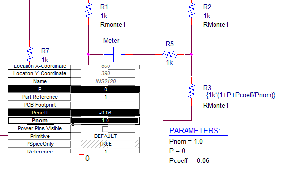
13. Edit the value property of R3 from 1K to {1K*(1+P+Pcoeff/Pnom)}.

 

14. Create a new simulation profile called Pressure.

 

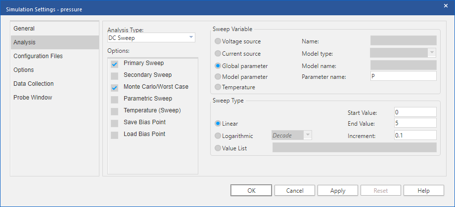
15. Configure a DC Sweep analysis of a global parameter P sweeping from 0 to 5 in 0.1 increments.

 

 

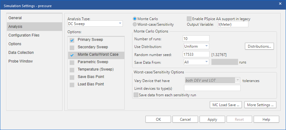
16. Left-click>Monte Carlo/Worst Case to enable the option.

 

17. Left-click on the Monte Carlo radio button. (rather than Worst Case)

 

18. Set the Output Variable to I(Meter).

 

19. Set the Number of runs to 10.

 

20. Set the Use distribution to Uniform by selecting it from the pull-down menu box.

 

21. Set the Random seed number to 17533.

 

22. Set Save data from to All by selecting it from the pull-down menu.

 

 

23. Left-click>OK to save and close the simulation profile.

 

24. Run the simulation.

Since the Monte Carlo analysis resulted in multiple simulation results, the prompt for “which results” is displayed, in this case the default, “all” will be selected.

 

25. When the Probe window opens after simulation, left-click>OK to select all of the data sections for viewing.

 

26. Left-click the Add Trace toolbar button, or use Trace>Add Trace from the top menu

 

27. Select I(Meter) from the list

 

28. Left-click>OK to add the trace.

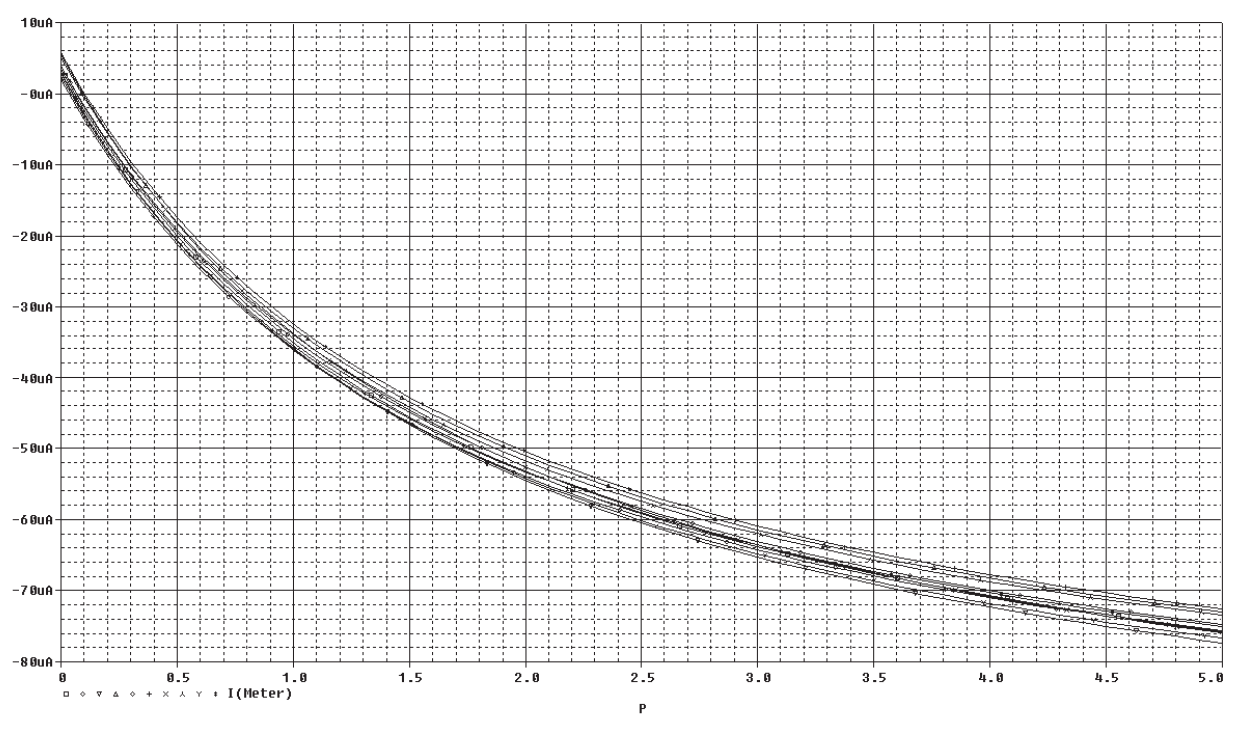
Note the variation on the displayed waveform caused by the variance introduced by the Monte Carlo analysis.

You can also look at the detailed results in the output file.

Partial listing of the output file follows:

* SORTED DEVIATIONS OF I(V_Meter) TEMPERATURE = 27.000 DEG C

MONTE CARLO SUMMARY

Mean Deviation = 603.2900E-09

Sigma = 1.8176E-06

RUN MAX DEVIATION FROM NOMINAL

Pass 6 3.0887E-06 (1.70 sigma) higher at P = 5 ( 95.914% of Nominal)

Pass 4 2.5897E-06 (1.42 sigma) higher at P = 5 ( 96.574% of Nominal)

Pass 8 2.1609E-06 (1.19 sigma) higher at P = 5 ( 97.141% of Nominal)

Pass 7 2.0296E-06 (1.12 sigma) higher at P = 0 ( 158.18% of Nominal)

Pass 3 1.7078E-06 ( .94 sigma) lower at P = 5 ( 102.26% of Nominal)

Pass 5 1.4642E-06 ( .81 sigma) lower at P = 0 ( 58.025% of Nominal)

Pass 9 1.0940E-06 ( .60 sigma) lower at P = 5 ( 101.45% of Nominal)

Pass 10 1.0088E-06 ( .56 sigma) lower at P = 0 ( 71.08 % of Nominal)

Pass 2 835.5300E-09 ( .46 sigma) higher at P = 5 ( 98.895% of Nominal)

 

 

End of Lab

 

 

All content Copyright 2022 Parallel Systems Ltd.