All content Copyright 2022 Parallel Systems Ltd.

 

1. Open the project named Buffer from previous labs

 

2. Open the Probe window with PSpice>View Simulation Results. Since the simulation data was created earlier, we don’t need to run the simulation again.

 

3. Add the trace I(CAP2).

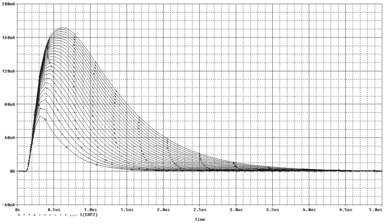
A measurement will be created that will measure the width of each trace. The pulse width will be defined as the difference between the X values of the trace measured at the 50% of each maximum Y value.

The Measurement Name will be PW, it will take a trace name as the single argument, the marked point expression will be x2-x1 (greater X value minus the lesser X value), there will need to be two search functions. The first will search for the 50% point of the trace on a positive slope, the second will search for the 50% point on the negative slope.

 

4. In the Probe window, choose Trace>Measurements.

 

5. Left-click>New in the Measurements dialog.

 

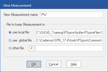
6. Type PW in the New Measurement Name field.

 

7. Check the Use Local File radio button. This will store the new measurement in a .prb file that has the same name as the active simulation profile.

 

8. Left-click>OK.

 

 

9. In the Edit New Measurement dialog, type the Marked Expression as x2-x1.

 

10. Change the search function to read

1| search forward level (50%,p) !1

search forward level (50%,n) !2;

Note

You must always place a semi-colon after the end of the entire function, not at the end of each search!

 

11. Left-click>OK to save the function and Close to close the dialog.

 

12. Left-click the Performance Analysis toolbar button.

 

13. Left-click the Trace Add toolbar button.

 

14. Scroll down the list of measurements and left-click to select PW (just created)

 

15. Left-click on the trace name I(CAP2) and it will be placed in the argument position of PW in the Trace Expression field.

 

16. Left-click>OK to add the trace.

 

17. Leave the Probe Window open with the PW function displayed for the next exercise.

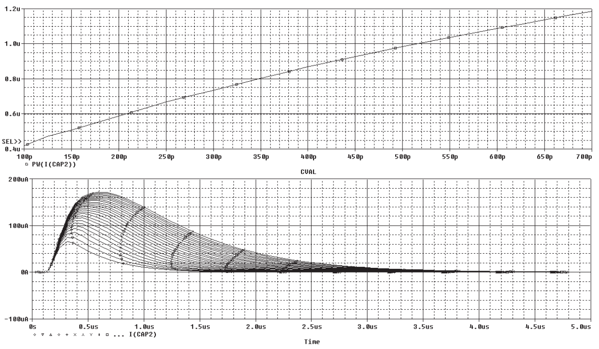
From the PW results, see that the pulse width of the current increases as the value of CAP2 increases. This was a simple example, but the steps are the same for a more difficult function.

a) Decide what you want to measure.

b) Examine the waveforms you have in order to determine which points on the trace will be needed to calculate the measured value.

c) Compose the search commands to find and mark the desired points.

d) Use the marked points in the Marked Point Expressions to calculate the final value for the trace.

e) Test the search commands and measurements.

 

 

End of Lab

 

 

All content Copyright 2022 Parallel Systems Ltd.